P3P Solutions
Visualizing Related Solution
Points for the P3P Problem
(http://www.mqrieck.com/P3P/P3P_Solutions.html)
M. Q. Rieck
(michael.rieck@drake.edu)
Last updated: April 17, 2024
The General Case
The Perspective 3-Point Pose (P3P) Problem is a camera tracking problem involving only three known control points to help locate the position of a camera. If you do not yet understand the P3P Problem, then perhaps you should seek out an introductory discussion first, for instance:
this. The following system of equations, due to J. A. Grunert, algebraically describes the P3P Problem:
r22 + r32 - 2c1r2r3 = d12
r32 + r12 - 2c2r3r1 = d22
r12 + r22 - 2c3r1r2 = d32
where r1, r2, r3 are the unknown distances from the camera's optical center to the control points (known points in 3D); d1, d2, d3 are the known distances between the control points; and c1, c2, c3 are the known cosines of the viewing angles (at the optical center) between pairs of control points. It will be helpful, henceforth, to assume that a Cartesian coordinate system (x,y,z) has been chosen for which the three control points all lie on the unit circle in the xy-plane.
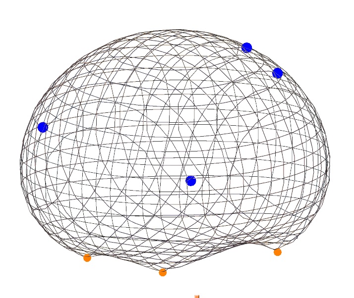
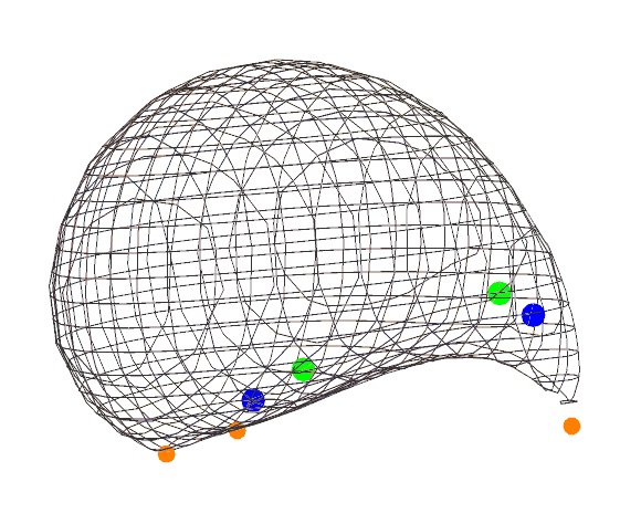
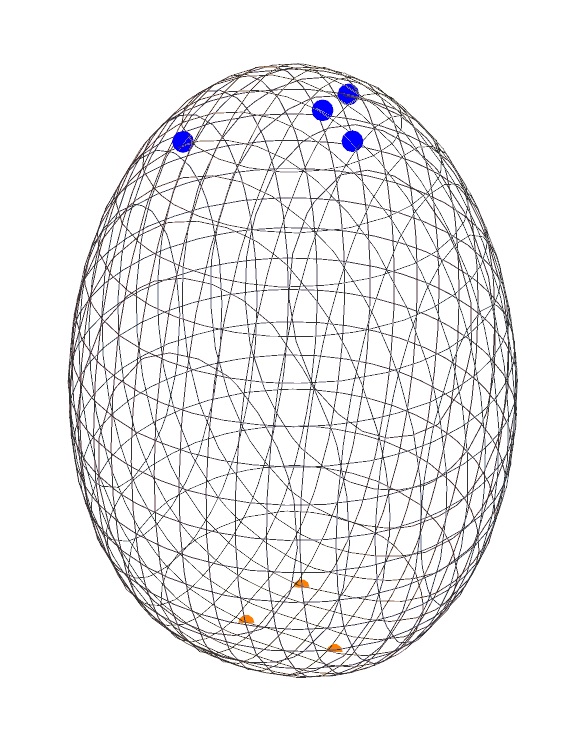
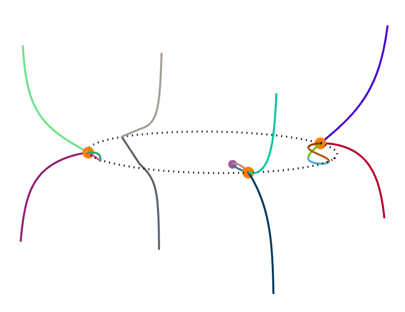
The above animation shows the three control points as orange dots. The blue dots are locations in space that have the same viewing angles of the control points, taken in pairs. These points solve the P3P system of equations using the same parameters, that is, the same d's and c's. Therefore, a knowledge of these parameters alone is insufficient to determine which of the blue positions is the actual position of the camera.
The green dots, when they occur, are such that the absolute values of the cosines of their viewing angles (|c1|, |c2|, |c3|) agree with those of the blue dots, but exactly two of the pairs of the corresponding cosines differ in sign. In other words, exactly two of the viewing angles at a green dot are the supplements of the corresponding viewing angles at a blue dot.
In the discussion to follow, the control points are fixed, and so the d's are just constants. For given values of the c's, certain points in space are solution points for this instance of the P3P Problem, i.e. for these P3P parameters.
Conversely, by considering any non-control point in space, there are unique values of the c's for which this point is one of the solution point of the P3P problem. In this way, you can say that the point determines an instance of the P3P Problem.
Thus, it is sometimes useful to consider the c's as functions of a point (x,y,z) in space.
When two points have the same viewing angles, and so the same values for the c's, that is, when they give the same instance of the P3P Problem,
these points are said to be (strongly) related (or isogonal). When they at least have the same absolute values of the c's, and when they differ in an even number (zero or two) of the c's, they will be said to be weakly related (or weakly isogonal).
In the above animation, all blue points are related to each other, but a blue point and a green point are only weakly related to each other. Note that (strongly) related implies weakly related, but not vice-versa. Notice too that two points are weakly related if and only if they have the same values of
c12, c22, c32
and c1c2c3.
There is a way to think about "weakly related" that is quite useful. By allowing the r's to be negative, one can regard that a point (x,y,z) with cosine values c1, c2, c3 and distance values r1, r2, r3 is also a "weak" solution point for the P3P Problem whose cosine values are instead c1, -c2, -c3, by using -r1, r2, r3 as signed distance values. This sort of thinking certainly complicates the discussion a bit, in a sense. However, "weakly related" can actually simplify the analysis because it allows for certain mathematical aspects to be handled in a continuous way that would otherwise not be possible.
For given parameters, all (weak) P3P solution points lie on a common surface that is either the control points plane or else a sixth degree algebraic surface that generally has "feet" on the control points, and is sometimes egg-shaped. Here are three examples:
A basic understanding of how related P3P solution points are situated in physical space can be found in a paper by Rieck and Wang [10], at least when the control points triangle is acute.
On the Control Points Plane
A very special case of the P3P Problem is the two-dimensional version, where the camera and the control points are coplanar. The situation here is rather well understood, but is by no means trivial. There is at most one other related solution point, and it must also be in the control points plane.
The above animation shows two moving dots, either two blue dots or else a blue dot and a green dot, at any given moment. These dots are said to be antigonal conjugates of each other, and their mathematical relation to each other can be characterized in several different ways. When there are two blue dots, they have exactly the same viewing angles of the three control points, and hence are (strongly) related P3P solution points. But when one of the moving dots is green, then two of the three pairs of corresponding viewing angles are supplementary, not equal. In this case, the two points are only weakly related.
(See D. M. Bailey [1], J. Van Yzeren [14] and Maienschein & Rieck [3]).
On an Altitude Plane
An altitude plane is obtained by taking one of the three altitude lines of the control points triangle, and extending it perpendicular to the control points plane. The case where the camera is located on an altitude plane has also been studied, in particular by W. J. Wolfe, D. Mathis, C. W. Sklair and M. Magee [13]. Here is an animation for this case that shows the orthogonal projections of the solution points onto the control points plane.
Near a Control Point
If one of the P3P solution points is infinitesimally close to one of the control points p, then the other solution points (and weak solution points) will be infinitesimally close to the double toroidal surface obtained by rotating the circumcircle of the control points triangle about the sideline opposite to p. This case has been studied by L. Hu, B. Wang and J. Zhang [2] and by B. Wang, H. Hu and C. Zhang [11]. It is also demonstrated in the following animation.
The Limit Case
Another interesting and important special case that has been studied is the limit case, where the camera is moved increasingly far away from the control points, in such a way that its orthogonal projection onto the control points plane stays fixed. That is, |z| goes to infinity, while fixing x and y. (See Rieck, 2015 [5])
To simplify the analysis, it is assumed (w.l.o.g.) that the circumcircle of the control points triangle is the unit circle in the xy-plane, and the triangle is oriented in a certain way. This amounts to requiring that the control points have coordinates (cos φ1, sin φ1, 0), (cos φ2, sin φ2, 0) and (cos φ3, sin φ3, 0), where φ1 + φ2 + φ3 = 0.
This keeps the triangle's orthocenter inside the so-called standard deltoid curve, as seen in the following animation (black dots = control points, purple dot = orthocenter):
 When the triangle is acute, the orthocenter is inside the triangle. When the triangle is obtuse, the orthocenter is outside the circumcircle.
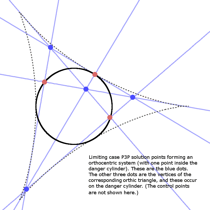
If the camera's projection onto the xy-plane (one of the blue points below) is inside the deltoid curve, but not on the danger cylinder, then there will be three other related solution points with the same property, and exactly one of the four points will be inside the danger cylinder. Together, the projections of these four points onto the control points plane form an orthocentric system (the blue dots; you can ignore the reddish dots, which are the vertices of the corresponding orthic triangle):
Moreover, in the limit case, the orthogonal projections of the mutually related solution points onto the control points plane can be characterized as the points of intersection of a pencil (family) of rectangular hyperbolas. This can be seen in the following animations, for three different cases. The various hyperbolas in each pencil are actually linear combinations of two fundamental hyperbolas. In the animation, we see a changing hyperbola that is a linear combination of the two fixed hyperbolas.
Here is another useful animation for the limit case that I will explain briefly. When it is inside the deltoid, the red triangular dot is the orthocenter of the triangle whose vertices are the orange triangular dots, which are on the unit circle, in this case. Identifying the xy-plane with the complex plane, the six black dots are the square roots (as complex numbers) of the orange dots. Certain triples of these form the vertices of four triangles whose orthocenters are the blue dots. These blue dots form an orthocentric system, and they are the orthogonal projections onto the xy-plane of the (related) P3P solution points, in the limit case. The green dots are the vertices of the orthic triangle for this orthocentric system. They are also the reflections of the orange dots about the y-axis, as long as the red dot is inside the deltoid. (Ignore the red circles.)
The General Case Again
Note: Much of the content of this and the next sections is more cleanly described
in Rieck and Wang [10]
and my preprint [8],
using complex numbers.
Returning now to the general P3P problem, there is a way to generalize the above results concerning rectangular hyperbolas, by using a quantity W, which is actually the varying quantity (x2+y2-1) / z2. However, in the limit case (above), W is just the constant zero. When approaching the control points plane instead, while staying off of the danger cylinder, W goes to infinity. The role played by the circumcircle when W = 0 is instead played by the nine-point circle of the control points triangle when W goes to infinity.
Here are some precise statements concerning the general P3P problem, where the spatial coordinate system is assumed to have been selected to facilitate the computations, and where Q = 1 / (1+W).
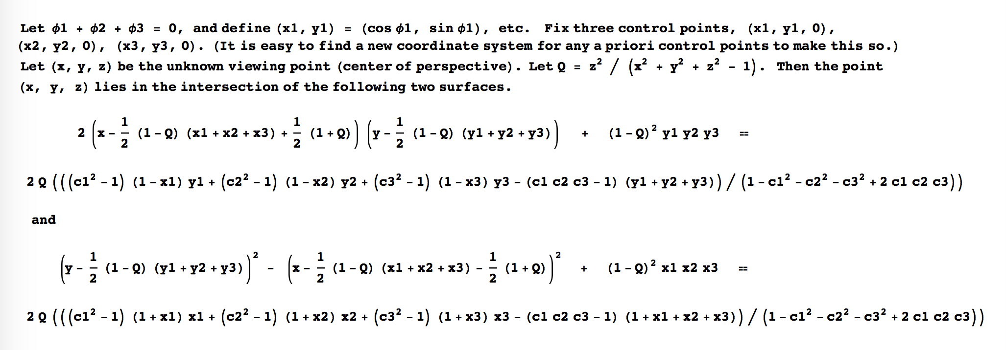
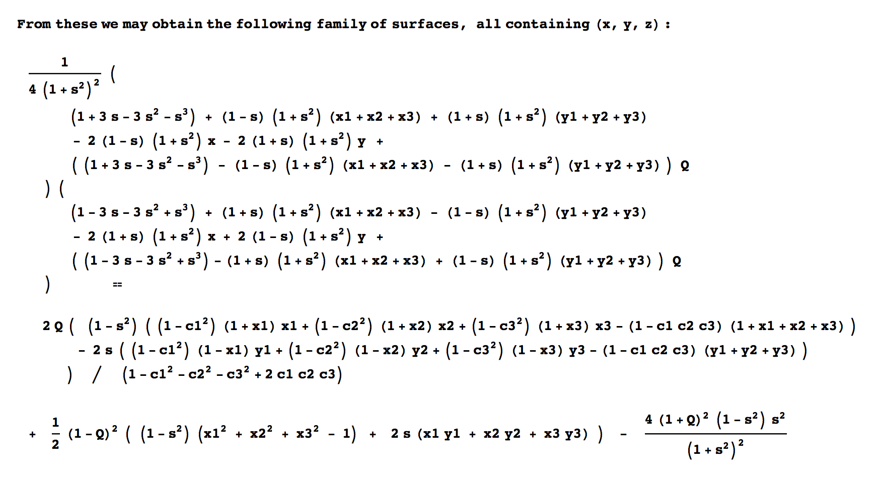
For any camera position not on the control points plane, the above describes some interesting surfaces that each pass through this point and all of its related solution points, and that tend to go through the control points too. These surfaces can be characterized as being precisely the contour surfaces of degree-one rational function in c12, c22, c32 and c1c2c3, expressed in terms of x, y and z, that converge non-trivially as |z| tends to infinity. As |z| goes to infinity, cross sections of these surfaces tend towards the rectangular hyperbolas of the limit case (see previous section).
Each of the following figures shows three of these special surfaces through the same related solution points, among an infinite family of such. The related solution points are not shown, but they all lie along the intersections of the surfaces, i.e. along the black curves in the figures. Points on such a curve have the same values of L and R, as defined in the next section.

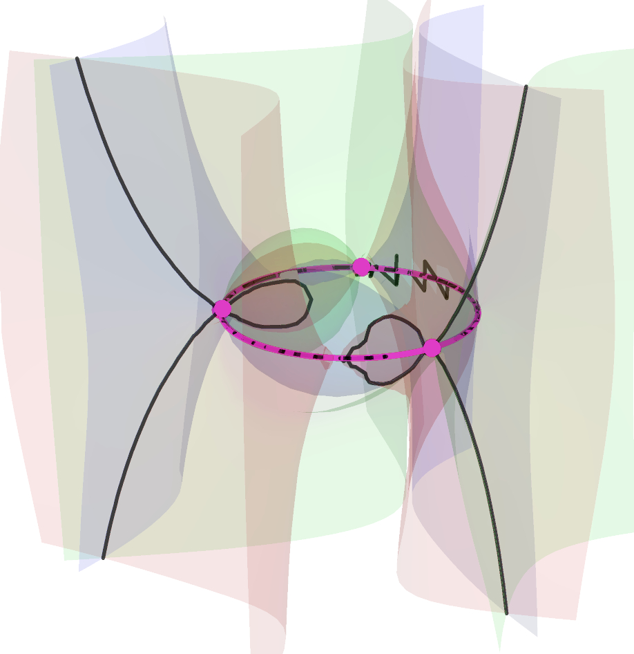
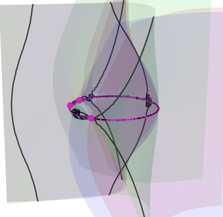
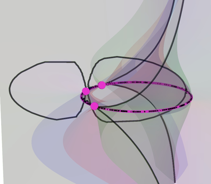
The wobbling and flickering near the circumcircle is mainly an artifact of the imprecision of the image rendering technique. The images below reveal more accurately the behavior of the curves near the control points plane, where the purple dots are the orthocenters, and significant portions of the curve have been colored differently.

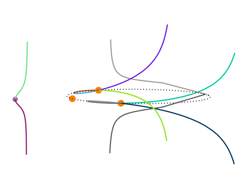
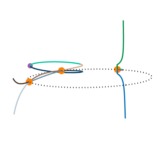
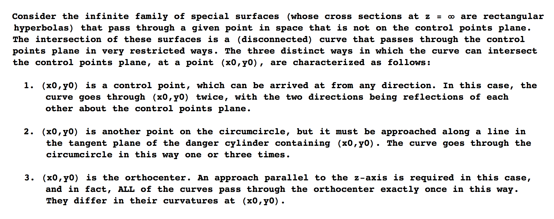
The following facts concerning the curves have been observed and proven:
The Discriminant
By taking the partial derivative of the left side of each of the three equations in Grunert's system, with respect to each of the three r's (with c's varying), we form a 3-by-3 Jacobian matrix J. To obtain the discriminant of Grunert's system, one can simply append the equation det(J) = 0 to the system and then eliminate the r's from the resulting system. This yields a single equation in the c's and d's. The equation originally seemed quite complicated, but it can be considerably tamed as follows.
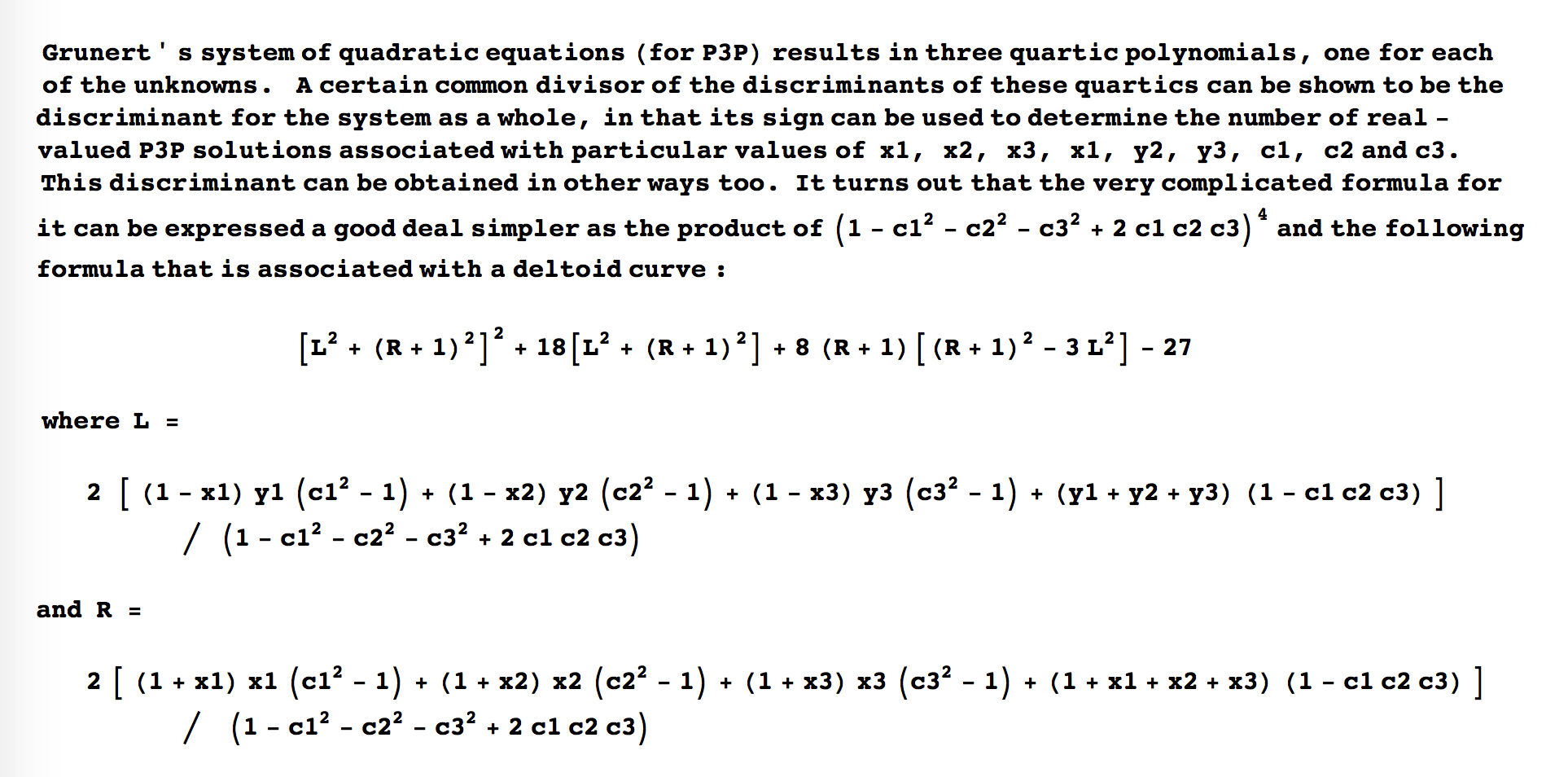
The x's and y's here are as in the previous sections. Recently, Bo Wang et al. [12] found a simpler way to express the above formula:
(L2 + R2 - 10R - 2)2 - 4 (1 - 2R)3.
Notice that weakly related points have the same values of c12, c22, c32, and c1c2c3, and therefore have the same
values of L and R. There is another interesting formula for the discriminant, in the case where the control points form an equilateral triangle, as follows:
4(1-c1c2c3)2(1+8c1c2c3)(1-c12-c22-c32+2c1c2c3) - 3(1+4c1c2c3-3c22c32-3c32c12-3c12c22+4c12c22c32)2.
Although it is not yet clear to what extent this formula extends to the general setup, there are a couple reasons to suspect that a nice generalization does exist.
A P3P solution point is a multiple (repeated) solution point if and only if it is on the danger cylinder surface. This is the cylinder obtained from the circumcircle of the control points triangle by extended it perpendicular to the control points plane. The discriminant of Grunert's system vanishes if and only if some solution point is on the danger cylinder.
One might then ask, which other points are weakly related to a point on the danger cylinder? Such points occur on a certain surface that mostly surrounds the danger cylinder.
The surface on which the discriminant of Grunert's system is zero is simply the union of this surface and the danger cylinder. Here are animations of this surface (half of it, actually, and without the danger cylinder) when the control points triangle is acute
(left) and when it is obtuse (right):
The surface has "feet" at the control points and at the orthocenter of the control points triangle. Much of the this material was introduced in a 2018 article by Rieck [6]. There the above surface is called the deltoidal surface, but in later papers,
[8],
[10] and
[12],
it is called the companion surface of the danger cylinder (CSDC).
Projections onto Control Points Plane
For the general P3P setup, the orthogonal projections of the (weak) P3P solution points onto the control points plane all lie on a nice cubic curve. Let us call this the circumcubic curve since it also passes through the control points. It also passed through the orthocenter of the control points triangle, and has asymptotes that are perpendicular to the triangle sides. For given P3P parameters, a portion of the circumcubic curve is actually the projection onto the xy-plane of the special (constant-L & constant-R) space curves discussed earlier.
The following is an animation that shows some of these circumcubic curves (blue), for various positions of the control points (black), and for various values of the parameters L and R. The orthocenter and altitude lines are shown too (orange).
Here is the equation of the circumcubic curve, for the parameters L and R, where (XH, YH) =
(x1 + x2 + x3, y1 + y2 + y3)
are the coordinates of the orthocenter of the control points triangle:
YH x3
+ (3 - XH) x2 y
+ YH x y2
- (XH + 1) y3
- (YH + L) x2
- 2 (XH + R + 1) x y
+ (YH + L) y2
+ (L XH + R YH - YH + L) x
+ (R XH + 3 XH - L YH - R - 1) y
+ (R YH + YH - L XH)
= 0.
Now, identify the xy-plane with the complex plane. Set ζ = x + i y, ζH = XH + i YH and ζL = - R - 1 + i L.
The discriminant can be written as follows:
ζL2 ζL2
- 4 (ζL3 + ζL3)
+ 18 ζL ζL
- 27.
The equation of the circumcubic curve can be written thus:
ζ3 - ζ3
- ζH ζ2 ζ
+ ζH ζ ζ2
+ (ζL - ζH) ζ2
+ (ζH - ζL) ζ2
+ (2 ζH + ζL - ζH ζL) ζ
+ (ζH ζL - 2 ζH - ζL) ζ
+ ζH ζL
- ζH ζL
= 0.
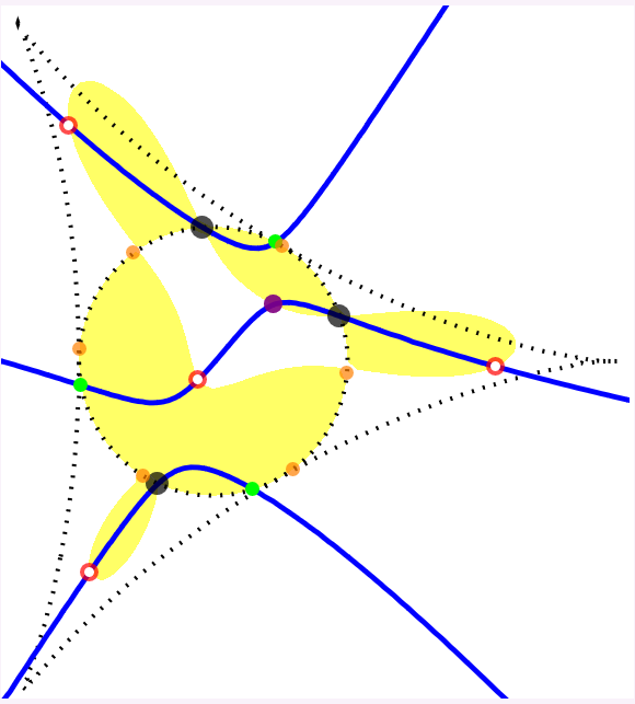
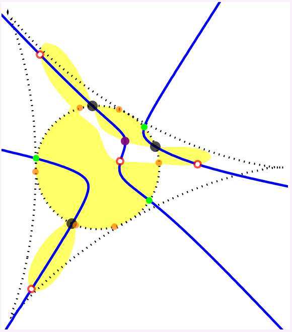
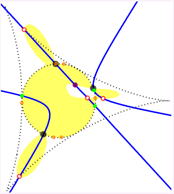
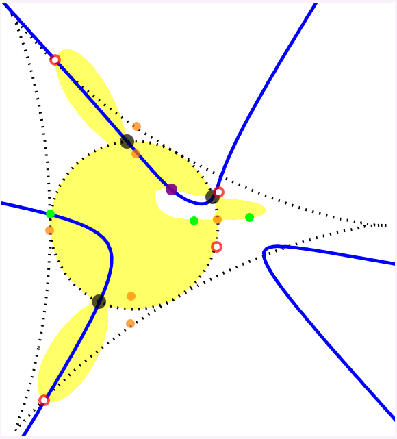
The following figures each show the circumcubic curve (blue), along with the control points (black dots), the orthocenter (purple dot), the negative conjugates of the roots ξ1, ξ2 and ξ3 of the complex cubic polynomial
ζ3 - ζL ζ2 + ζL ζ - 1 (green dots),
the square roots of these cubic polynomial roots, ± ω1, ± ω2 and ± ω3 (orange dots; ω1 ω2 ω3 = 1),
and the points
χ0 = ω1 + ω2 + ω3,
χ1 = ω1 - ω2 - ω3,
χ2 = - ω1 + ω2 - ω3 and
χ3 = - ω1 - ω2 + ω3 (red and white dots).
In the first three figures, the discriminant is negative, and the four red (and white) dots are the orthogonal projections, onto the xy-plane, of the four (weak) solution points for the limit case.
In the last figure, the discriminant is positive, and only the two red (and white) dots on the circumcubic curve correspond to (weak) solution points in the limit case.
When the discriminant is negative, the four red (and white) dots form an orthocentric system, and the green dots are the vertices of the corresponding orthic triangle.
The latter are also intersection points for the circumcubic curve and the circumcircle of the control points triangle.
The yellow region is where the circumcubic curve is the projection onto the xy-plane of the constant-ζL space curve.
There are also quartic curves (like the blue curve in next figure) that pass through the projections of the (weak) P3P solution points onto the xy-plane, the control points and the orthocenter of the control points triangle. Let us call these curves, the circumquartic curves. Like the circumcubic curve (gray in the next figure), they have some other interesting properties (not spelled out here).
Note: A detailed analysis of the discriminant and the points discussed here can be found in my preprint [8].
Note: Using the pn notation in my preprint [9], the complex numbers
χ0, χ1, χ2 and χ3 are related to the complex number ζL via
p2(χ0) = p2(χ1) = p2(χ2) = p2(χ3) = ζL.
Here, p2(z) = z2 - 2 z for complex numbers z.
Miscellaneous Deltoid Constructions
This section is just "fun with deltoids," and is not necessarily relevant to P3P. In the following figure, on the left, the orange diamond marks a point that determines a unique (orange) triangle, and as long as this point stays inside the standard deltoid, the triangle's vertices are on the unit circle and its orthocenter is the point marked by the orange diamond.
This triangle determines a doubly infinite family of relate triangles with vertices on the unit circle and orthocenters inside the deltoid. Treating the vertices of the original triangle as complex numbers of norm one, the other triangles are obtained by raising these numbers to the same integer power. A few of the resulting triangles are seen on the left, along with their orthocenters. On the right, we see several more of these triangle vertices and orthocenters. Here the red diamond takes the place of the orange diamond on the left.
More about this can be found in my preprint [9],
which you might consult if you get interested in the following challenges.
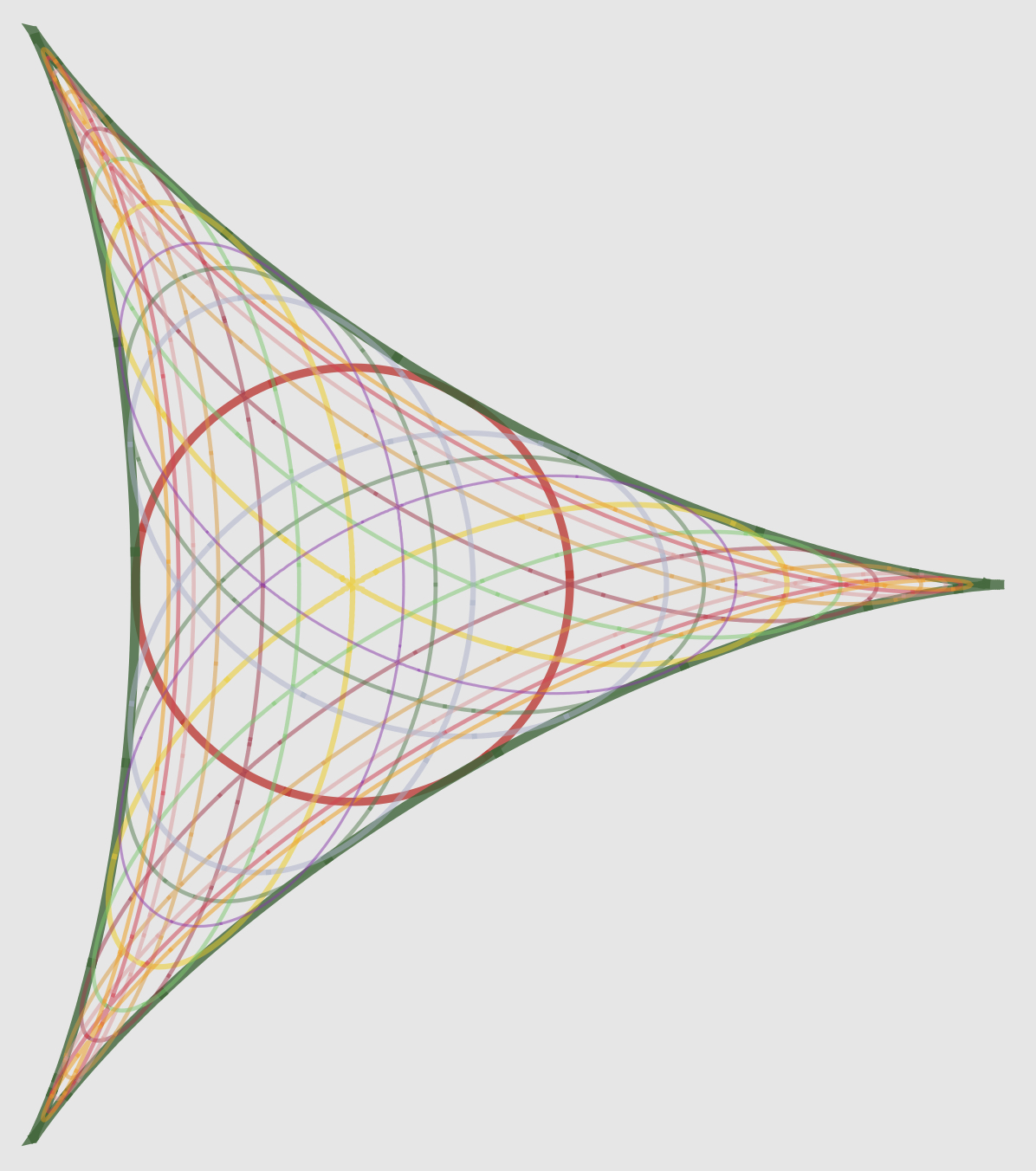
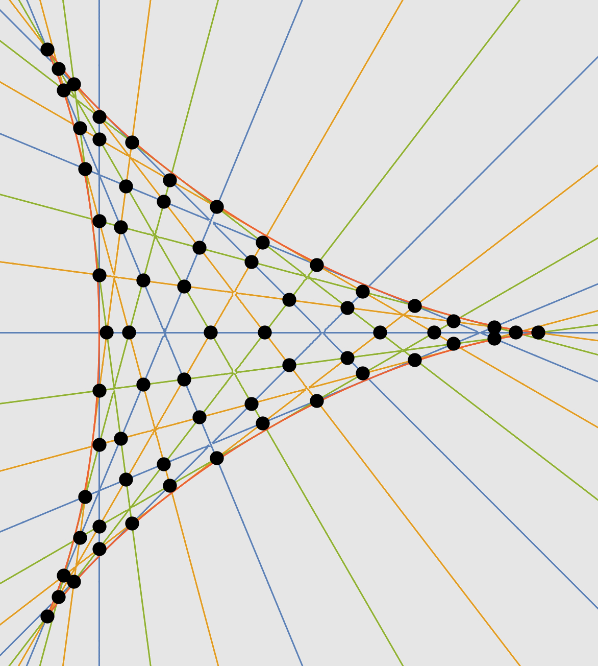
Challenge 1: The next figure includes some members of a family of curves that are dense in the interior of the deltoid and that have a connection with the construction in triangle geometry discussed above.
Basically, if we start at a point on one of these curves, regarded as a triangle orthocenter, then infinitely many of the triangles described above will collapse (be degenerate triangles) and have their orthocenters on the deltoid. With or without this insight, figure out what these curves are and how to draw them.
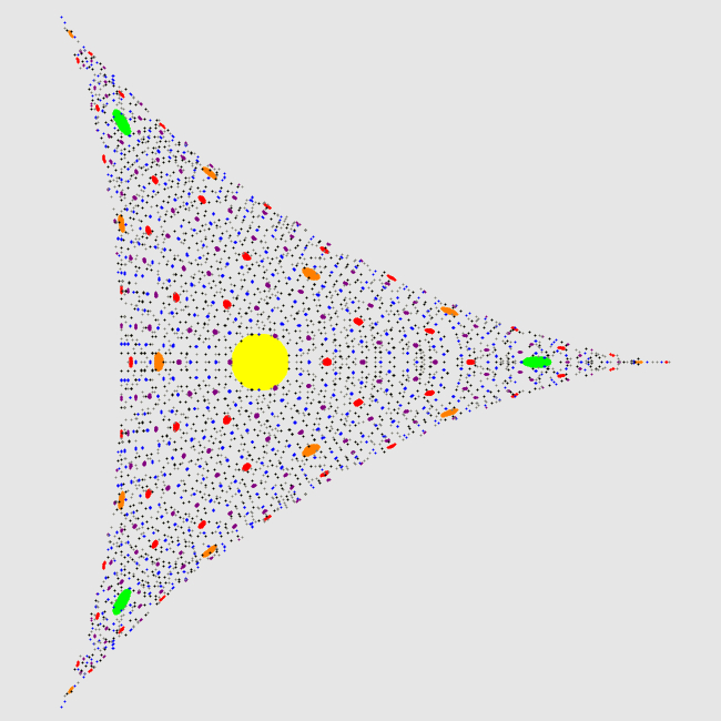
Challenge 2: When the orthocenter of one of the triangles considered here is at the center of the deltoid, then the triangle is equilateral. The next figure shows how certain points, regarded as triangle orthocenters, get mapped to points near the center, when triangle vertices, considered as complex numbers, are repeatedly squared.
The yellow region just shows points within a certain distance of the center. The green region shows points for which the "squaring map" results in a point in the yellow region. The orange region shows points for which the "squaring map" results in a point in the green region. And so forth.
Can you see how to describe all the points that are eventually mapped to the center of the deltoid? Such points
are the orthocenters of triangles for which repeatedly squaring the triangle vertices eventually produces an equilateral triangle.
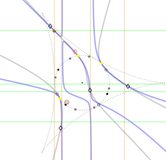
Challenge 3: Figure out about the parallel lines in the following animated figure.
Challenge 4: The tangent lines to the deltoid are
quite significant. Figure out what is being communicated
in these last two figures. Actually, I'll explain the marked intersection points in the figure on the right. These are the orthocenters of triangles for which "raising to the eighth power" transforms the vertices of the original triangle to an equilateral triangle (whose center is at the center of the deltoid).
References
- D. M. Bailey: "Some reflective geometry of the triangle," Math. Magazine, 33(5), 241-259 (1960)
-
L. Hu, B. Wang, J. Zhang: "Singular points in the optical center distribution of p3p solutions," Mathematical Problems in Engineering, 2015, #147397, 6 pages
-
T. D. Maienschein, M. Q. Rieck: "Angular coordinates and rational maps," J. Geometry and Graphics, 20(1), 41-62 (2016) (available here)
-
M. Q. Rieck: "A fundamentally new view of the perspective 3-point pose problem," J. Math. Imaging and Vision, 48(3), 499-516 (2014) (available here)
-
M. Q. Rieck: "Related solutions to the perspective three-point pose problem," J. Math. Imaging and Vision, 53(2), 225-232 (2015) (available here)
-
M. Q. Rieck: "On the discriminant of Grunert's system of algebraic equations and related issues," J. Math. Imaging and Vision, 60(5), 737-762 (2018) (available here)
-
M. Q. Rieck: "Four problems in solid geometry with proposed solutions," preprint (2022)
(available here)
-
M. Q. Rieck: "Understanding the deltoid phenomenon in the perspective 3-point (p3p) problem," preprint (2023)
(available here)
-
M. Q. Rieck: "The deltoid curve and triangle transformations," Int. J. Geom., 13(1), 78-91 (2024)
(available here)
-
M. Q. Rieck, B. Wang: "Locating perspective three-point problem solutions in spatial regions," J. Math. Imaging and Vision, 63(8), 953-973 (2021) (available here)
-
B. Wang, H. Hu, C. Zhang: "New insights on multi-solution distribution of the p3p problem," preprint, arXiv:1901.11464v1 (2019)
-
B. Wang, H. Hu, C. Zhang: "Companion surface of danger cylinder and its role is solution variation of p3p problem," preprint, arXiv:1906.08598v1 (2019)
-
W. J. Wolfe, D. Mathis, C. W. Sklair, M. Magee: "The perspective view of three points," IEEE Trans. Pattern Analysis and Machine Learning, 13(1), 66-73 (1991)
-
J. Van Yzeren: "Antigonal, isogonal and inverse," Math. Magazine, 65(5), 339-347 (1992)